the last question
How to Land on the Moon
June 30, 2025
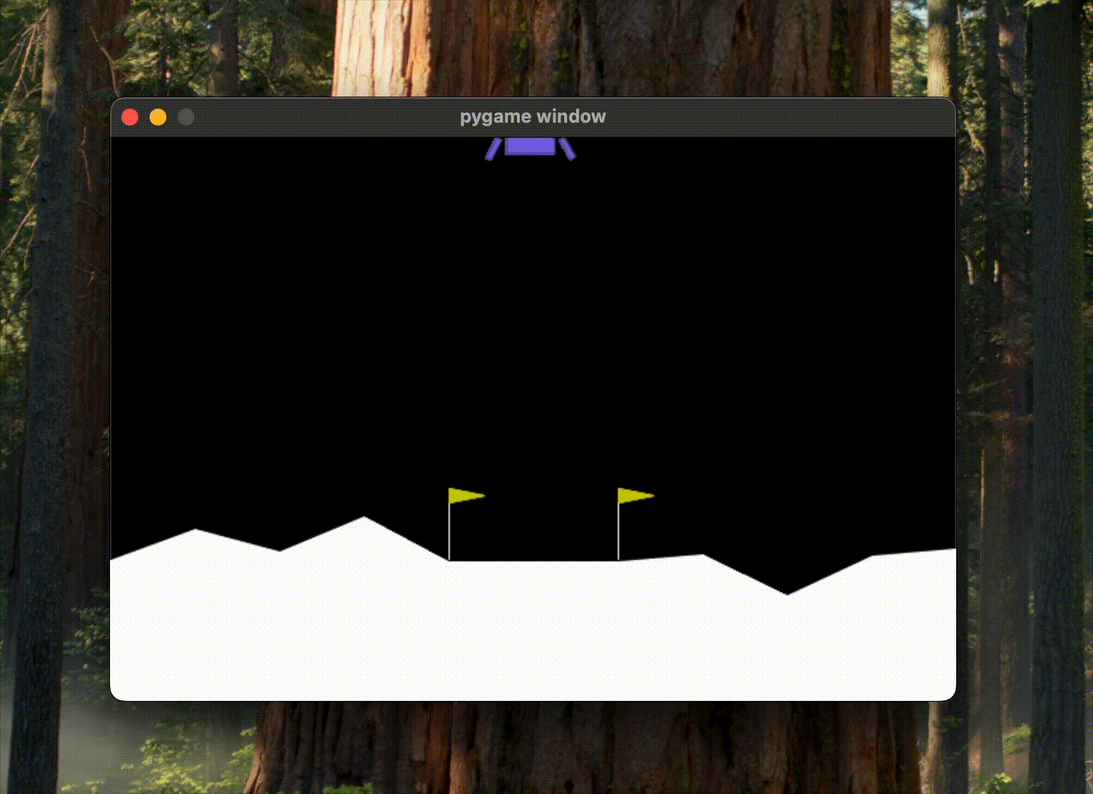
Wanted to land the thing. First attempts would avoid crashing sometimes, which felt like progress. But not landing.
The lander learned to hover. Just hover perfectly, draining fuel until the episode timed out. 100+ points for doing nothing. RL is dumb like that.
Got it working eventually. Code.
This is how
I ran eight environments in parallel. The rewards are sparse, so you need a lot of data before anything shows up.
env_name = 'LunarLanderContinuous-v3'
state_dim, action_dim = 8, 2
num_envs = 8
I scaled the observations the way the docs suggest.
OBS_SCALE = np.array([10, 6.666, 5, 7.5, 1, 2.5, 1, 1], dtype=np.float32)
One network with two heads: eight layers for the actor, four for the critic.
class ActorCritic(nn.Module):
    def __init__(self, state_dim, action_dim, hidden_dim, actor_layers, critic_layers):
        super(ActorCritic, self).__init__()

        actor = [nn.Linear(state_dim, hidden_dim), nn.ReLU()]
        for _ in range(actor_layers - 1):
            actor.extend([nn.Linear(hidden_dim, hidden_dim), nn.ReLU()])
        actor.append(nn.Linear(hidden_dim, action_dim))
        self.actor = nn.Sequential(*actor)
        self.log_std = nn.Parameter(torch.zeros(action_dim))

        critic = [nn.Linear(state_dim, hidden_dim), nn.ReLU()]
        for _ in range(critic_layers - 1):
            critic.extend([nn.Linear(hidden_dim, hidden_dim), nn.ReLU()])
        critic.append(nn.Linear(hidden_dim, 1))
        self.critic = nn.Sequential(*critic)

    def forward(self, state):
        action_mean = self.actor(state)
        action_std = self.log_std.exp()
        value = self.critic(state)
        return action_mean, action_std, value
log_std is a parameter too, so the network learns how much to explore on its own.
Sample from the Gaussian, squash through tanh to keep the actions in range. The squash bends the probability density, so you have to correct for it:
def tanh_log_prob(raw_action, dist):
    action = torch.tanh(raw_action)
    logp_gaussian = dist.log_prob(raw_action).sum(-1)
    return logp_gaussian - torch.log(1 - action**2 + 1e-6).sum(-1)
That last term is the log-determinant of the tanh Jacobian.
class PPO:
    def __init__(self, actor_critic, pi_lr, vf_lr, gamma, lamda, K_epochs, eps_clip,
                 batch_size, vf_coef, entropy_coef):
        self.actor_critic = actor_critic
        self.states, self.actions = [], []
        self.pi_optimizer = optim.Adam(
            list(actor_critic.actor.parameters()) + [actor_critic.log_std],
            lr=pi_lr
        )
        self.vf_optimizer = optim.Adam(actor_critic.critic.parameters(), lr=vf_lr)
        self.gamma, self.lamda, self.K_epochs = gamma, lamda, K_epochs
        self.eps_clip, self.batch_size = eps_clip, batch_size
        self.vf_coef, self.entropy_coef = vf_coef, entropy_coef
The actor learns at 3e-4, the critic at 1e-3.
PPO clips the probability ratio (Schulman et al.):
\[L^{CLIP}(\theta) = \mathbb{E}_t \left[ \min \left( r_t(\theta) \hat{A}_t, \text{clip}(r_t(\theta), 1-\varepsilon, 1+\varepsilon) \hat{A}_t \right) \right]\]Where \(r_t(\theta) = \frac{\pi_\theta(a_t \mid s_t)}{\pi_{\theta_{\text{old}}}(a_t \mid s_t)}\).
The clip keeps the policy from jumping too far in one update.
def compute_loss(self, batch_states, batch_actions, batch_logprobs,
                 batch_advantages, batch_returns):
    action_means, action_stds, state_values = self.actor_critic(batch_states)
    dist = torch.distributions.Normal(action_means, action_stds)
    action_logprobs = tanh_log_prob(batch_actions, dist)
    ratios = torch.exp(action_logprobs - batch_logprobs)

    actor_loss = -torch.min(
        ratios * batch_advantages,
        torch.clamp(ratios, 1-self.eps_clip, 1+self.eps_clip) * batch_advantages
    ).mean()
    critic_loss = F.mse_loss(state_values.squeeze(-1), batch_returns)
    entropy = dist.entropy().sum(-1).mean()

    return actor_loss + self.vf_coef * critic_loss - self.entropy_coef * entropy
The loss is the clipped objective, plus value MSE, minus an entropy bonus. One backward pass feeds both optimizers.
Advantages via GAE:
def compute_advantages(self, rewards, state_values, is_terminals):
    T, N = rewards.shape
    advantages, gae = torch.zeros_like(rewards), torch.zeros(N, device=rewards.device)
    state_values_pad = torch.cat([state_values, state_values[-1:]], dim=0)

    for t in reversed(range(T)):
        delta = rewards[t] + self.gamma * state_values_pad[t + 1] * (1 - is_terminals[t]) - state_values_pad[t]
        gae = delta + self.gamma * self.lamda * (1 - is_terminals[t]) * gae
        advantages[t] = gae

    returns = advantages + state_values_pad[:-1]
    advantages = (advantages - advantages.mean()) / (advantages.std() + 1e-8)
    return advantages.reshape(-1), returns.reshape(-1)
GAE (Schulman et al.):
\[\hat{A}_t^{GAE(\gamma,\lambda)} = \sum_{l=0}^{\infty} (\gamma \lambda)^l \delta_{t+l}^V\]Lambda is 0.95. Normalize the advantages or the gradients blow up.
The rollout stores the raw actions, before the tanh:
def __call__(self, state):
    action_np, state_tensor, raw_action = self.actor_critic.act(
        state, deterministic=False, return_internals=True
    )
    self.states.append(state_tensor)
    self.actions.append(raw_action)
    return action_np
All eight environments step together:
def rollout(env, policy, num_steps=None, num_episodes=None):
    states, _ = env.reset()
    traj_rewards, traj_dones = [], []
    ep_returns, ep_rets, step_count = [], np.zeros(env.num_envs), 0

    while True:
        states, rewards, terminated, truncated, _ = env.step(policy(states))
        traj_rewards.append(rewards)
        traj_dones.append(np.logical_or(terminated, truncated))
        ep_rets += rewards
        step_count += env.num_envs

        if np.any(traj_dones[-1]):
            for idx in np.where(traj_dones[-1])[0]:
                ep_returns.append(ep_rets[idx])
                ep_rets[idx] = 0.0

        if (num_steps and step_count >= num_steps) or
           (num_episodes and len(ep_returns) >= num_episodes):
            break

    return traj_rewards, traj_dones, ep_returns
100k steps per epoch, then 20 update passes over them at batch size 5000:
def update(self, rewards, dones):
    with torch.no_grad():
        rewards = torch.as_tensor(np.stack(rewards), dtype=torch.float32).to(device)
        is_terms = torch.as_tensor(np.stack(dones), dtype=torch.float32).to(device)
        old_states, old_actions = torch.cat(self.states), torch.cat(self.actions)
        action_means, action_stds, old_state_values = self.actor_critic(old_states)
        old_logprobs = tanh_log_prob(old_actions,
                                     torch.distributions.Normal(action_means, action_stds))
        old_state_values = old_state_values.squeeze(-1).view(-1, rewards.size(1))
        advantages, returns = self.compute_advantages(rewards, old_state_values, is_terms)

    dataset = TensorDataset(old_states, old_actions, old_logprobs, advantages, returns)
    for _ in range(self.K_epochs):
        for batch in DataLoader(dataset, batch_size=self.batch_size, shuffle=True):
            batch_states, batch_actions, batch_logprobs, batch_advantages, batch_returns = batch

            self.pi_optimizer.zero_grad()
            self.vf_optimizer.zero_grad()

            loss = self.compute_loss(batch_states, batch_actions, batch_logprobs,
                                    batch_advantages, batch_returns)
            loss.backward()

            torch.nn.utils.clip_grad_norm_(
                list(self.actor_critic.actor.parameters()) + [self.actor_critic.log_std],
                max_norm=0.5
            )
            torch.nn.utils.clip_grad_norm_(self.actor_critic.critic.parameters(), max_norm=0.5)

            self.pi_optimizer.step()
            self.vf_optimizer.step()

    self.states, self.actions = [], []
Gradients clipped at 0.5.
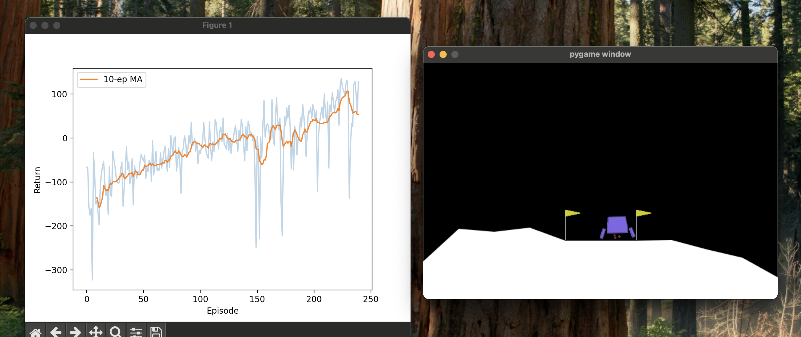
I evaluate every 10 epochs:
def evaluate_policy(actor_critic, n=16, render=False, num_episodes=None):
    env = make_env(1 if render else n, render)
    def policy(s): return actor_critic.act(s, deterministic=True)

    if render and num_episodes:
        _, _, ep_rets = rollout(env, policy, num_episodes=num_episodes)
    else:
        _, _, ep_rets = rollout(env, policy, num_steps=max_timesteps * (1 if render else n))

    env.close()
    return float(np.mean(ep_rets)) if ep_rets else 0.0
It stops when the moving average hits 250, which takes about 100 epochs.
One small step for the optimizer, one giant leap for the GPU bill.